Graph of the Day

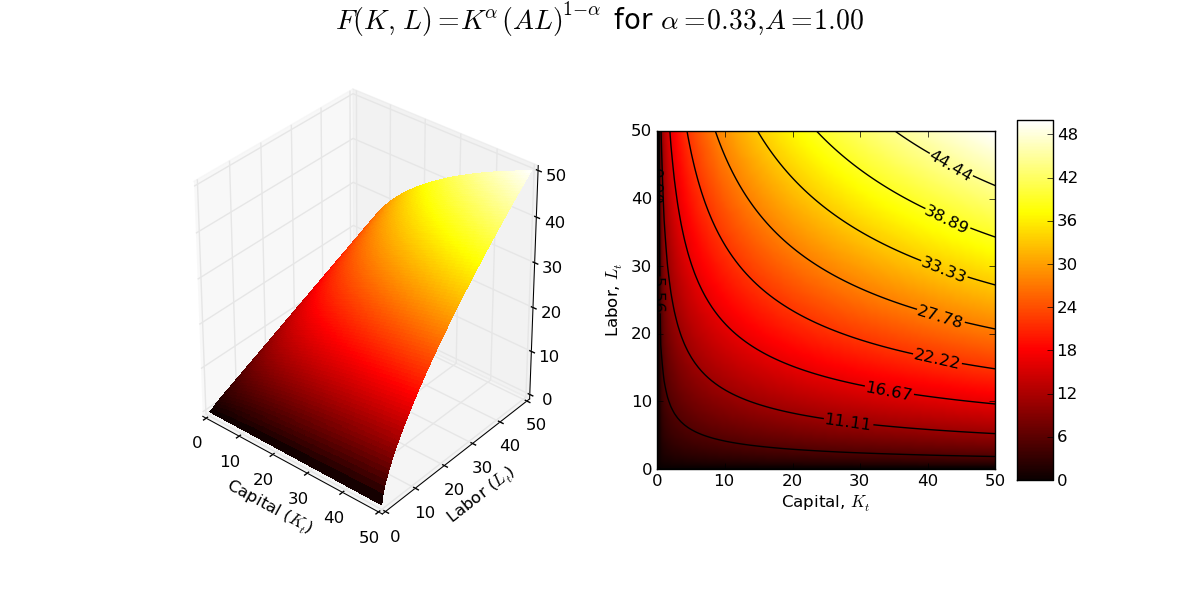
Today's graph is a combined 3D plot of the production frontier associated with the constant returns to scale Cobb-Douglas production function and a contour plot showing the isoquants of the production frontier. This static snapshot was written up using matplotlib (the code also includes an interactive version of the 3D production frontier implemented in Mayavi).

At some point I will figure out how to embed the interactive Mayavi plot into a blog post so that readers can manipulate the plot and change parameter values. If anyone knows how to do this already, a pointer would be much appreciated!