α-Stable Distributions and Extreme Value Theory...

Below is a slightly edited excerpt from my MSc Thesis...

Fat-Tails and α-Stable Distributions: There is now a large, and growing, body of literature documenting the “fat-tail” properties of a number of economic variables (i.e., stock returns, oil and other commodity prices, income, exchange rates, etc.)  In the event that the "fat-tail" of a given variable follows a power law, such variables may be well described  by α-stable distributions.  Such distributions are sometimes also referred to as α-Levy stable distributions after the mathematician Paul Levy who first characterized the class of distributions in 1924 as part of his study of normalized sums of i.i.d. terms.  An intriguing property of α-stable distributions is that they will often exhibit an infinite variance.  Seminal work in applying α-stable distributions to economic variables, stock prices and commodity prices, is Fama (1963, 1965a, 1965b) and Mandlebrot (1961, 1963, 1967).

α-Stable distributions are described by four parameters:

1. α - the stability parameter (sometimes called the index of stability or characteristic exponent), which takes values in the range (0,2]
2. β - a skewness parameter which takes values [-1,1]. If β>0 the distribution is skewed to the right, while if β<0 the distribution is skewed to the left.
3. c - a scale parameter which takes values (0, +∞)
4. μ - a location parameter which takes values (-∞, +∞). The location parameter shifts the entire distribution to the right if μ>0 and to the left if μ<0.

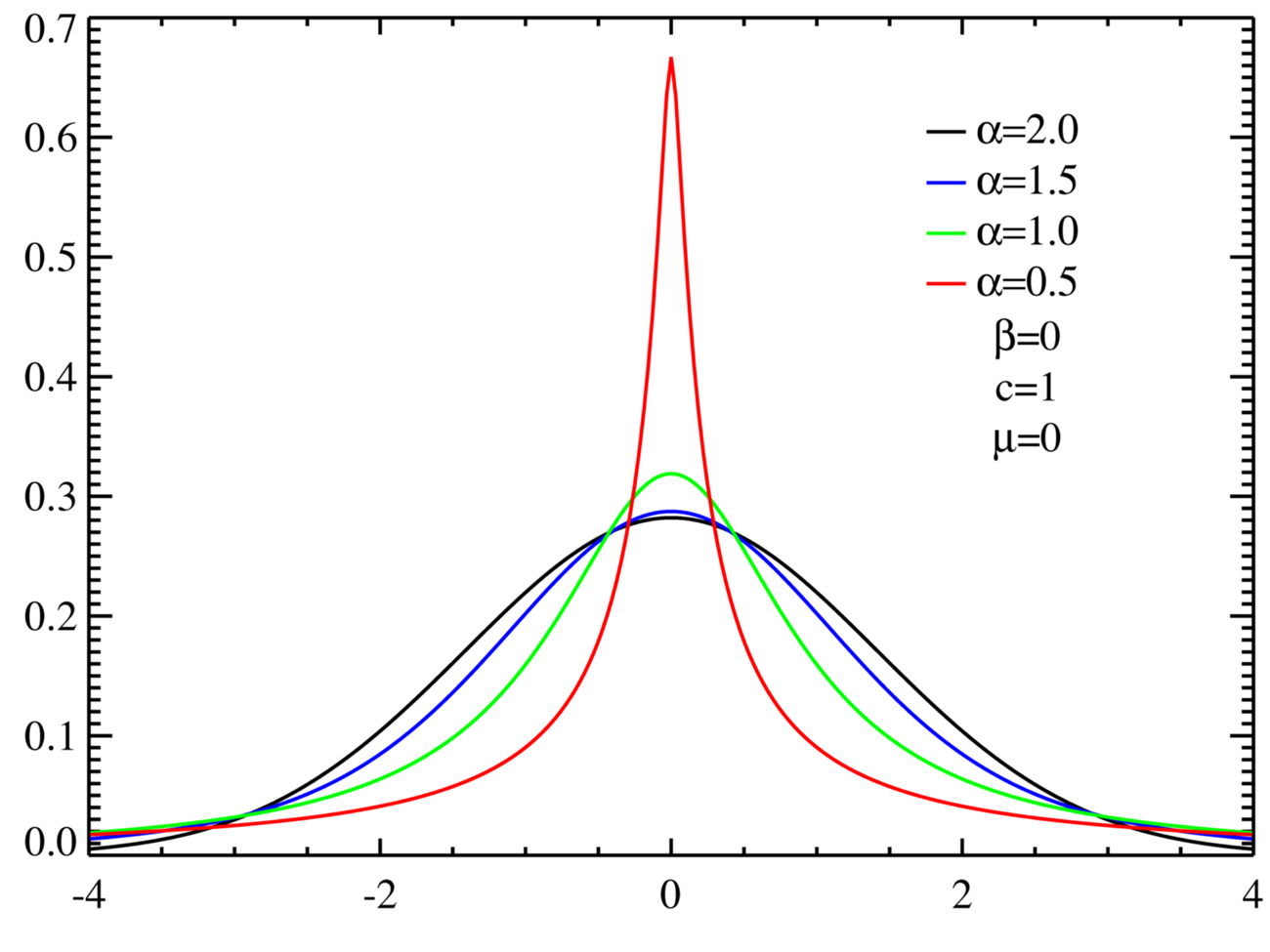
The class of α-stable distributions encompasses the more well known normal (Gaussian) and Cauchy distributions as special cases. The stable distribution with α=1 corresponds to the Cauchy distribution, whereas the case α=2 corresponds to a normal distribution. It is important to note that α-stable distributions with α<2 have an infinite variance, and that therefore the normal (Gaussian) distribution is the only stable distribution that has a finite variance.  Figure A.1 presents density plots of symmetric (β=0), centered (μ=0) α-stable distributions for α=0.5, 1.0, 1.5, 2.0. Note that in all cases the distributions have a unit scale factor (c=1). The case α=2.0 corresponds to the normal (Gaussian) distribution. The “fat-tail” behavior of α-stable distributions can easily be seen in Figure A.1.

Figure A.1: Theoretical Density plots of various α-stable distributions

The α-stable distributions are intimately connected to Pareto (power law) distributions: the tails of α-stable distributions are asymptotically Pareto (power law) distributed. Power laws turn up quite frequently in economics. Gabaix (2009) is an excellent review of power law distributions, their applications in economics, and their relationship to “fat-tail” behavior.

Why work with a distribution with an infinite variance? There are three reasons main reasons why one might want to use α-stable distributions in a model (Nolan 2009). First, there may be sound theoretical reasons to expect a particular economic process to be non-normal (Gaussian).  Gabaix (2009) provides several theoretical applications in economics and finance.  The second reason is that α-stable distributions have their own central limit theorem. The Generalized Central Limit Theorem, as stated in Nolan (2009), says that the only possible non-trivial limit of normalized sums of i.i.d terms must be an α-stable distribution. The third reason is empirical. As mentioned above there is a growing body of research documenting the “fat-tails” and skewness of many economic variables. The class of α-stable distributions allows the researcher to parsimoniously account for both the “fat-tail” and skewness characteristics of the data.

When I wrote this section of my thesis, I was more than a little bit enthralled with power laws and infinite variance (I blame it on too much time reading Taleb's the Black Swan).  Some caveats about what I wrote above based on what I have learned in the past year:

1. Power Law behavior implies fat-tails, but fat-tails doesn't necessarily imply power law behavior.
2. Just because a variable exhibits linear behavior when plotted on log-log scales, doesn't mean that it follows a power law.
3. Even if you find that your variable does follow a power-law, this doesn't necessarily mean that it is well described by a stable distribution.
4. Even if you find that your variable does follow a power-law, this doesn't mean that it must also have an infinite variance. 

When I look at economic time-series data, one of the things that always jumps out at me is the volatility of many key economic variables.  Often times significant portions of the total variation in the variable's time-series can be accounted for in only a hand full of extreme movements.  Such extreme movements by definition tend to occur in the extreme quantiles or “tail(s)” of the underlying probability distribution.  Classical statistical analysis techniques tend to be ill-suited for estimating the extreme quantiles of probability distributions.

In many critical real-world situations the events that are of most concern to the economic policy-maker are those events that have low-probability, high-impact events. Extreme Value Theory (EVT) is the branch of statistical theory that deals primarily with developing techniques to accurately (and more importantly consistently) estimate the shape of the extreme quantiles or tails of a distribution.  As the only class of limiting distributions for sums of i.i.d. random variables, α-stable distributions play a central role in a branch of statistics known as Extreme Value Theory (EVT).  However, the central result of Extreme Value Theory is the Fisher-Tippet theorem describing the limit behavior of the maxima, Mn, of an i.i.d sequence {Xn}.

The Fisher-Tippet Theorem says the following: given a sequence {Xn} of i.i.d random variables drawn from some common distribution F, define M1=0 and Mn=max{X1,…,Xn} for n≥2 (this is just a sequence of maximum events). If the distribution of Mn (after being appropriately re-centered and re-scaled) converges to some non-degenerate limit distribution H as n gets “large,” then H must be one of the following three distributions: the Fréchet, the Weibull, or the Gumbel.

These three distributions are known collectively as the Extreme Value Distributions and can be expressed by a single distribution called the Generalized Extreme Value (GEV) distribution Hξ. The parameter ξ defines the shape of the distribution in terms of tail “thickness.” The case where the shape parameter ξ>0 (“fat-tails”) corresponds to the Fréchet distribution, ξ=0 (“thin-tails”) corresponds to the Gumbel distribution, and when ξ<0 (“bounded-tails”) Hξ is the Weibull distribution.

In sum, as a result of some mathematical jiggery-pokery if we are interested in how extreme economic "events" behave, we can focus our attention on trying to fit one of the three Extreme Value distributions to the extreme events in our economic time series data.

Key Assumptions: Although the Fisher-Tippet theorem was derived for i.i.d. sequences, the convergence result also holds under fairly mundane regularity conditions and under less stringent assumptions than independence.  The key assumption that is required for the Fisher-Tippet theorem to hold is stationarity (i.e., the parameters of H are independent of time). Unfortunately for applications of EVT, the assumption of stationarity is often violated in real-world data. This is particularly relevant for economic data where stationarity of the data generating process (DGP) for our economic events would require that the “true” DGP for generating economic events also not change through time.  For a process as highly adaptive as that of economic activity, stationarity is simply not plausible (regardless of the result of formal statistical tests for time-series stationarity). When dealing with non-stationary data, current practice dictates that the researcher introduces time dependence in the extreme value parameters.

Crazy Side Note: It is my belief that there are two classes of non-stationary DGPs. Class-I non-stationary DGPS are those whose parameters are well described by some deterministic or mildly stochastic function of time.  In this situation, assuming that one correctly models the function describing the non-stationary behavior, techniques exist to estimate the relevant parameters and derive confidence intervals.  A key implicit assumption used to estimate Class-I non-stationary series is that the functional form that determines how the parameters change with time is, itself, time invariant.  If this implicit assumption is valid, then this would justify the use of historical data to forecast future events.

Class-II non-stationary DGPs, on the other hand are those whose parameters are constantly changing with time due to some underlying adaptive process. In this case even if one is willing to assume that the adaptive process can be modeled by some combination of deterministic and mildly stochastic components, the key implicit assumption of time invariance of the assumed functional form is clearly violated.  If one is dealing with a class 2 non-stationary DGP, then use of historical data to forecast future events is highly questionable.  Unfortunately, for us economists, the DGP for economic events is likely Class-II non-stationary.

References:

• Fama, E. 1963. “Mandelbrot and the Stable Paretian Hypothesis.” Journal of Business 36(4), 1963, 420–429.
• Fama, E. “Portfolio Analysis in a Stable Paretian Market.” Management Science 11(3A), 1965a, 404–419.
• Fama, E. “The Behavior of Stock Market Prices.” Journal of Business 38(1), 1965b, 34–105.
• Gabaix, Xavier. “Power Laws in Economics and Finance.” Annual Review of Economics, 1, 2009.
• Mandelbrot B. “Stable Paretian Random Functions and the Multiplicative Variation of Income.” Econometrica, 29, 1961, 517-43
• Mandelbrot, B. “The Variation of Certain Speculative Prices.” Journal of Business, 36, 1963, 394-419.
• Nolan, J. “Numerical Computation of Stable Densities and Distribution Functions.” Communications in Statistics-Stochastic Models, 15, 1997, 759-774.
• Nolan, J.P. “Stable Distributions – Models for Heavy Tailed Data.” Birkhauser, Forthcoming 2009. (Chapter 1 available online at http://academic2.american.edu/~jpnolan/stable/stable.html.)