How well do you know your utility function?

This is an excerpt from my teaching notes for an upcoming computational economics lab on the RBC model that I am teaching at the University of Edinburgh that I thought might be of more general interest (mostly because of the cool graphics!)...

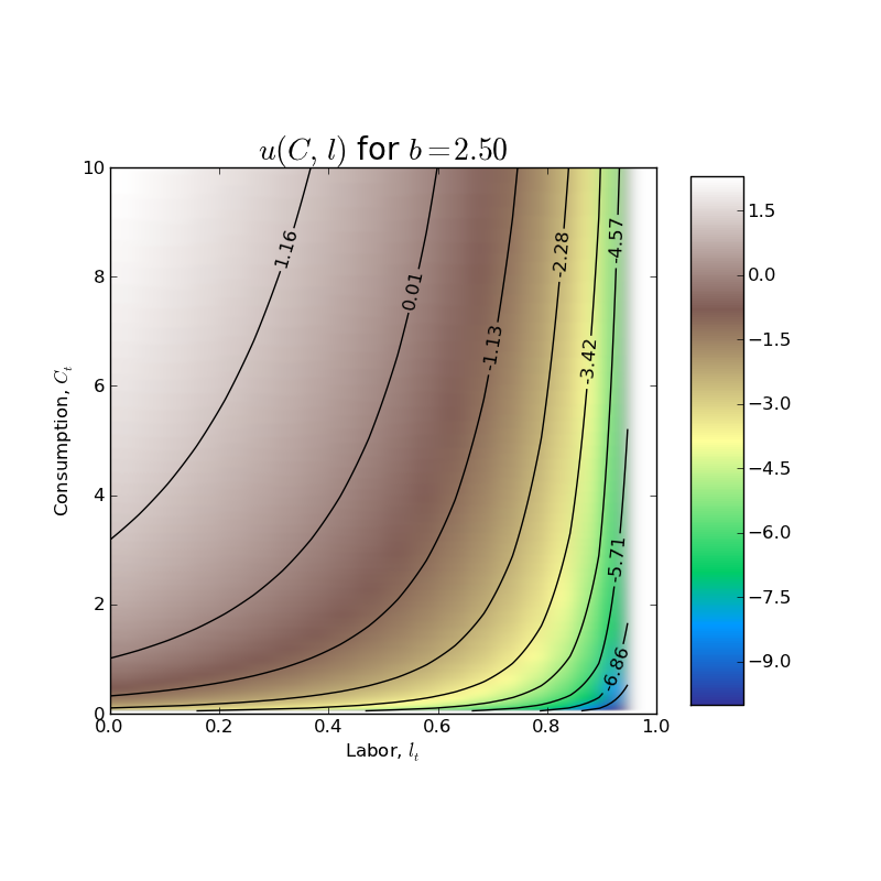
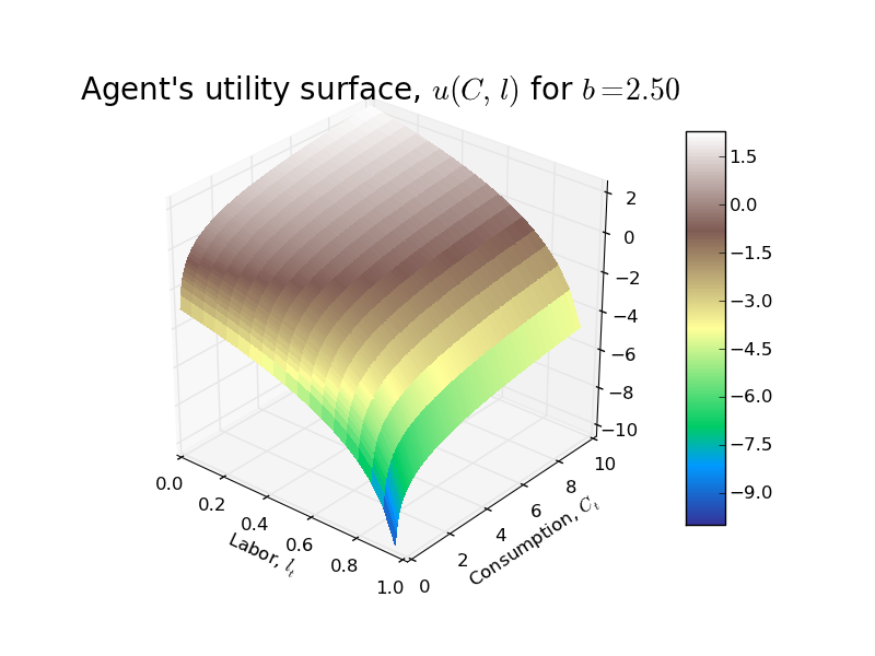
In the basic RBC model from Chapter 5 of David Romer's Advanced Macroeconomics, the representative household has the following single period utility function: $$u(C_{t}, l_{t}) = ln(C_{t}) + b\ ln(1 - l_{t})$$ where $C_{t}$ is per capita consumption, $l_{t}$ is labor (note that labor endowment has been normalized to 1!), and $b$ is a parameter (just a weight that the household places on utility from leisure relative to utility from consumption).

First a 3D plot of the utility surface...

Followed by a nice contour plot showing the indifference curves for the agent...

Suppose that the representative household lives for two periods and that there is no uncertainty about future prices.  Because of logarithmic preferences, the household will follow the decision rule 'consume a fraction fixed fraction of the PDV of lifetime net worth.'  We can derive this decision rule formally as follows. First, note that the household budget constraint is $$C_{0} + \frac{1}{1 + r_{1}}C_{1} = w_{0}l_{0} + \frac{1}{1 + r_{1}}w_{1}l_{1}$$ where $r_{1}$ is the real interest rate.  The Lagrangian for the household's two period optimization problem is $$\max_{\{C_{t}\}, \{l_{t}\}} ln(C_{0}) + b\ ln(1-l_{0}) + \beta[ln(C_{1}) + b\ ln(1-l_{1})] + \lambda\left[w_{0}l_{0} + \frac{1}{1 + r_{1}}w_{1}l_{1} - C_{0} - \frac{1}{1 + r_{1}}C_{1}\right]$$ The household now chooses sequences of consumption and labor (i.e., representative household chooses $C_{0}, C_{1}, l_{0}, l_{1}$). The FOC along with the budget constraint imply a system of 5 equations in the 5 unknowns $C_{0}, C_{1}, l_{0}, l_{1}, \lambda$ as follows: $$\begin{align}\frac{1}{C_{0}} - \lambda =& 0 \\ \beta\frac{1}{C_{1}} - \lambda \frac{1}{1+r_{1}}=& 0 \\-\frac{b}{1 - l_{0}} + \lambda w_{0} =& 0 \\-\beta\frac{b}{1 - l_{1}} + \lambda \frac{1}{1 + r_{1}}w_{1} =& 0 \\C_{0} + \frac{1}{1 + r_{1}}C_{1} =& w_{0}l_{0} + \frac{1}{1 + r_{1}}w_{1}l_{1}\end{align}$$ This 5 equation system can be reduced (by eliminating the Lagrange multiplier $\lambda$) to a linear system of 4 equations in 4 unknowns: $$\begin{vmatrix} b & \ 0 & \ w_{0} & 0 \\\ \beta(1 + r_{1}) & -1 & 0 & 0 \\\ 0 & \ b & 0 & w_{1} \\\ 1 & \frac{1}{1 + r_{1}} & -w_{0} & -\frac{1}{1+r_{1}}w_{1} \end{vmatrix} \begin{vmatrix}C_{0} \\\ C_{1} \\\ l_{0} \\\ l_{1}\end{vmatrix} = \begin{vmatrix} w_{0} \\\ 0 \\\ w_{1} \\\ 0\end{vmatrix}$$ The above system can be solved in closde form using some method like Cramer's rule/substitution etc to yield the following optimal sequences/policies for consumption and labor supply: $$\begin{align}C_{0} =& \frac{1}{(1 + b)(1 + \beta)}\left(w_{0} + \frac{1}{1 + r_{1}}w_{1}\right) \\ C_{1} =& \left(\frac{1 + r_{1}}{1 + b}\right)\left(\frac{\beta}{1 + \beta}\right)\left(w_{0} + \frac{1}{1 + r_{1}}w_{1}\right) \\ l_{0} =& 1 - \left(\frac{b}{w_{0}}\right)\left(\frac{1}{(1 + b)(1 + \beta)}\right)\left(w_{0} + \frac{1}{1 + r_{1}}w_{1}\right) \\ l_{1} =& 1 - \left(\frac{b\beta(1+r_{1})}{w_{1}}\right) \left(\frac{1}{(1 + b)(1 + \beta)}\right)\left(w_{0} + \frac{1}{1 + r_{1}}w_{1}\right) \end{align}$$
Several important points to note about the above optimal consumption and labor supply policies:

• Household's lifetime net worth, $w_{0} + \frac{1}{1 + r_{1}}w_{1}$, is the present discounted value of its labor endowment.
• Household's lifetime net worth depends on the wages in BOTH periods and future interest rate.  It hints at the more general result that, if the household has an infinite time horizon, lifetime net worth depends on the entire future path of wages and interest rates.
• In each period, household's consume a fraction of their lifetime net worth. Although the fraction changes in this simple two period model, if the household has an infinite horizon, the fraction of lifetime net worth consumed each period will be fixed and equal to $$\frac{1}{(1 + b)(1 + \beta + \beta^2 + \dots)}=\frac{1 - \beta}{1 + b}$$
• From the policy function for $l_{0}$, one can show that in order for the labor supply in period $t=0$ to be non-negative (which it must!), the following inequality must hold: $$\left(\frac{1}{1 + r_{1}}\right)\left(\frac{w_{1}}{w_{0}}\right) \lt \frac{(1 + b)(1 + \beta)}{b} - 1$$
• From the policy function for $l_{1}$, in order for the labor supply in period $t=1$ to be non-negative (which it must!), the following inequality must hold: $$(1 + r_{1})\left(\frac{w_{0}}{w_{1}}\right) \lt \left(\frac{1 + b}{b}\right)\left(\frac{1 + \beta}{\beta}\right) - 1$$

If we specify some prices (i.e., wages in period $t=0, 1$, $w_{0}=5,w_{1}=9$ and the interest rate $r_{1}=0.025$), then we can graphically represent the optimal choices of consumption and labor supply in period $t=0$ and $t=1$ as follows.

Note that with the wage in $t=1$ being almost twice as high as the wage in period $t=0$, the agent pushes his labor supply in period $t=0$, $l_{0}$, almost all the way to zero (i.e., he chooses not to work very much). The agent can still consume because, absent any frictions (things like borrowing constraints, incomplete markets, imperfect contracts, etc), he can easily consume some of his future labor earnings in period $t=1$ in the current period.

In period $t=1$, although the higher wage causes the agent to significantly increases his labor supply, there is no much change in his level of consumption (i.e., there is consumption smoothing!).

As always, code is available on GitHub.