For Those Interested in ABM...

I came across an excellent set of lecture slides from Daniel Katz at Michigan on computational modeling for social sciences, and for those interested in NetLOGO there are an excellent set of introductory tutorials on Youtube

Endogenous Business Cycles and Randomness...

As I was re-reading Masanao Aoki's Reconstructing Macroeconomics: A Perspective from Statistical Physics and Combinatorial Stochastic Processes, I came upon (again) an insight regarding the stochastic nature of business cycles that I think is worth sharing.  The insight was originally Eugene Slutsky's.  The basic idea is that the simple summation of random variables can produce cycles.  A concrete example will help fix ideas.  Suppose we have the following random walk model:

Si-Si-1=ei=+/-1 for all i=1,2,... with S0=0

with the respective probability of either outcome (i.e., -1 or 1) equal to a half.   This is simply a model of "winnings" from tossing a fair coin (where heads wins $1 and tails losses $1)  The unconditional mean of this process is zero, which might lead one to expect that the process spends "most" of the time "near" its zero unconditional mean.  But this intuition would be incorrect.  Take a look at the following diagram of a sample path of 10,000 tosses of a fair coin:

 

For me, Slutsky's insight should be taken as a reminder that quite sophisticated behavior, including cycles, can be generated out of simple randomness.  I actually think that this insight is more general than even Slutsky might have been willing to admit.  Simple randomness is a major force in this world, especially in economic behavior.  We as economists tend to be too quick to assume that the sophisticated/complicated macroeconomic behavior that we see in the world must be the result of fairly (or extremely) sophisticated human behavior at the micro level. 

Perhaps the macroeconomic behavior we observe is actually being driven by fairly simplistic humans operating by "rules of thumb" sprinkled with a bit of randomness...

Computational Modeling...

A nice simple set of lecture slides on computational modeling in the social sciences by Ken Kollman at Michigan (although I have to admit that the uninitiated will probably not find them terribly informative)...also I will have limited to no internet this week...expect fewer than normal posts.

Posting will resume apace from Edinburgh next Monday...

The Hidden Hazards of Adaptive Behavior...

James passed me this interesting paper on the stability of multivariate systems where agents use adaptive behavior via email.  I did a quick read...heavy on the maths (although I think it is mostly just multivariate calculus and linear algebra). They also went all out on the notation...I haven't seen some of those symbols outside of formal advanced maths texts. It would take quite a bit of work for me to fully grasp the paper as I would need to follow through on the calculations etc. Although plowing through the maths would be a good refresher...

I think his (i.e., James') characterization of the paper in the email is pretty much on target. They seem to formally develop general conditions under which multivariate systems with adaptive expectations are not stable. They find that for the most part, such systems are not stable.  And they stress that their results provide further evidence that equilibrium stability results from models where homogeneous agents are using adaptive behavior (or that are otherwise one-dimensional) should not be generalized to high dimensional or heterogeneous agent models where agents are using adaptive behavior.  The study of multivariate (and heterogeneous agent) systems, would seem to be a study in disequilibrium behavior...

Their results support the other research on multivariate and complex adaptive systems that I have read. From my reading of the literature, multivariate systems (including heterogeneous agent systems), generally speaking, are not stable.  At least in the sense that it is rare that such complex systems settle down to some static equilibrium.  On the other hand many multivariate and complex adaptive systems do exhibit endogenous self-organizing behavior (which I like to think of as a type of stable disequilibrium behavior...although this may not be the best choice of words to capture the phenomenon), punctuated equilibrium dynamics, etc.

The more I learn about economics, the more I am becoming convinced that economics is not an equilibrium science.  Economics is fundamentally a science of disequilibrium behavior.  I will go out on a limb here and say that perhaps one of the reasons that economics, particularly macroeconomics, has struggled so much is because we as economists are trying to force our (for the most part) linear equilibrium models to describe a non-linear disequilibrium world...

There is also the (I'd like to think small) possibility that I am cocooned in a world of complex adaptive systems, and am suffering from a massive case of confirmation bias...

α-Stable Distributions and Extreme Value Theory...

Below is a slightly edited excerpt from my MSc Thesis...

Fat-Tails and α-Stable Distributions: There is now a large, and growing, body of literature documenting the “fat-tail” properties of a number of economic variables (i.e., stock returns, oil and other commodity prices, income, exchange rates, etc.)  In the event that the "fat-tail" of a given variable follows a power law, such variables may be well described  by α-stable distributions.  Such distributions are sometimes also referred to as α-Levy stable distributions after the mathematician Paul Levy who first characterized the class of distributions in 1924 as part of his study of normalized sums of i.i.d. terms.  An intriguing property of α-stable distributions is that they will often exhibit an infinite variance.  Seminal work in applying α-stable distributions to economic variables, stock prices and commodity prices, is Fama (1963, 1965a, 1965b) and Mandlebrot (1961, 1963, 1967).

α-Stable distributions are described by four parameters:

1. α - the stability parameter (sometimes called the index of stability or characteristic exponent), which takes values in the range (0,2]
2. β - a skewness parameter which takes values [-1,1]. If β>0 the distribution is skewed to the right, while if β<0 the distribution is skewed to the left.
3. c - a scale parameter which takes values (0, +∞)
4. μ - a location parameter which takes values (-∞, +∞). The location parameter shifts the entire distribution to the right if μ>0 and to the left if μ<0.

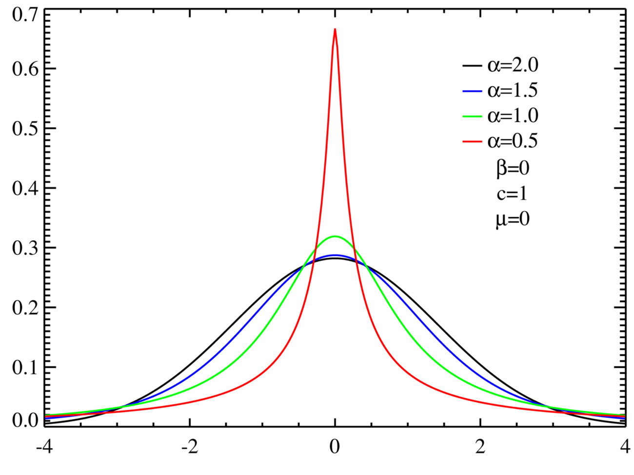
The class of α-stable distributions encompasses the more well known normal (Gaussian) and Cauchy distributions as special cases. The stable distribution with α=1 corresponds to the Cauchy distribution, whereas the case α=2 corresponds to a normal distribution. It is important to note that α-stable distributions with α<2 have an infinite variance, and that therefore the normal (Gaussian) distribution is the only stable distribution that has a finite variance.  Figure A.1 presents density plots of symmetric (β=0), centered (μ=0) α-stable distributions for α=0.5, 1.0, 1.5, 2.0. Note that in all cases the distributions have a unit scale factor (c=1). The case α=2.0 corresponds to the normal (Gaussian) distribution. The “fat-tail” behavior of α-stable distributions can easily be seen in Figure A.1.

Figure A.1: Theoretical Density plots of various α-stable distributions

The α-stable distributions are intimately connected to Pareto (power law) distributions: the tails of α-stable distributions are asymptotically Pareto (power law) distributed. Power laws turn up quite frequently in economics. Gabaix (2009) is an excellent review of power law distributions, their applications in economics, and their relationship to “fat-tail” behavior.

Why work with a distribution with an infinite variance? There are three reasons main reasons why one might want to use α-stable distributions in a model (Nolan 2009). First, there may be sound theoretical reasons to expect a particular economic process to be non-normal (Gaussian).  Gabaix (2009) provides several theoretical applications in economics and finance.  The second reason is that α-stable distributions have their own central limit theorem. The Generalized Central Limit Theorem, as stated in Nolan (2009), says that the only possible non-trivial limit of normalized sums of i.i.d terms must be an α-stable distribution. The third reason is empirical. As mentioned above there is a growing body of research documenting the “fat-tails” and skewness of many economic variables. The class of α-stable distributions allows the researcher to parsimoniously account for both the “fat-tail” and skewness characteristics of the data.

When I wrote this section of my thesis, I was more than a little bit enthralled with power laws and infinite variance (I blame it on too much time reading Taleb's the Black Swan).  Some caveats about what I wrote above based on what I have learned in the past year:

1. Power Law behavior implies fat-tails, but fat-tails doesn't necessarily imply power law behavior.
2. Just because a variable exhibits linear behavior when plotted on log-log scales, doesn't mean that it follows a power law.
3. Even if you find that your variable does follow a power-law, this doesn't necessarily mean that it is well described by a stable distribution.
4. Even if you find that your variable does follow a power-law, this doesn't mean that it must also have an infinite variance. 

When I look at economic time-series data, one of the things that always jumps out at me is the volatility of many key economic variables.  Often times significant portions of the total variation in the variable's time-series can be accounted for in only a hand full of extreme movements.  Such extreme movements by definition tend to occur in the extreme quantiles or “tail(s)” of the underlying probability distribution.  Classical statistical analysis techniques tend to be ill-suited for estimating the extreme quantiles of probability distributions.

In many critical real-world situations the events that are of most concern to the economic policy-maker are those events that have low-probability, high-impact events. Extreme Value Theory (EVT) is the branch of statistical theory that deals primarily with developing techniques to accurately (and more importantly consistently) estimate the shape of the extreme quantiles or tails of a distribution.  As the only class of limiting distributions for sums of i.i.d. random variables, α-stable distributions play a central role in a branch of statistics known as Extreme Value Theory (EVT).  However, the central result of Extreme Value Theory is the Fisher-Tippet theorem describing the limit behavior of the maxima, Mn, of an i.i.d sequence {Xn}.

The Fisher-Tippet Theorem says the following: given a sequence {Xn} of i.i.d random variables drawn from some common distribution F, define M1=0 and Mn=max{X1,…,Xn} for n≥2 (this is just a sequence of maximum events). If the distribution of Mn (after being appropriately re-centered and re-scaled) converges to some non-degenerate limit distribution H as n gets “large,” then H must be one of the following three distributions: the Fréchet, the Weibull, or the Gumbel.

These three distributions are known collectively as the Extreme Value Distributions and can be expressed by a single distribution called the Generalized Extreme Value (GEV) distribution Hξ. The parameter ξ defines the shape of the distribution in terms of tail “thickness.” The case where the shape parameter ξ>0 (“fat-tails”) corresponds to the Fréchet distribution, ξ=0 (“thin-tails”) corresponds to the Gumbel distribution, and when ξ<0 (“bounded-tails”) Hξ is the Weibull distribution.

In sum, as a result of some mathematical jiggery-pokery if we are interested in how extreme economic "events" behave, we can focus our attention on trying to fit one of the three Extreme Value distributions to the extreme events in our economic time series data.

Key Assumptions: Although the Fisher-Tippet theorem was derived for i.i.d. sequences, the convergence result also holds under fairly mundane regularity conditions and under less stringent assumptions than independence.  The key assumption that is required for the Fisher-Tippet theorem to hold is stationarity (i.e., the parameters of H are independent of time). Unfortunately for applications of EVT, the assumption of stationarity is often violated in real-world data. This is particularly relevant for economic data where stationarity of the data generating process (DGP) for our economic events would require that the “true” DGP for generating economic events also not change through time.  For a process as highly adaptive as that of economic activity, stationarity is simply not plausible (regardless of the result of formal statistical tests for time-series stationarity). When dealing with non-stationary data, current practice dictates that the researcher introduces time dependence in the extreme value parameters.

Crazy Side Note: It is my belief that there are two classes of non-stationary DGPs. Class-I non-stationary DGPS are those whose parameters are well described by some deterministic or mildly stochastic function of time.  In this situation, assuming that one correctly models the function describing the non-stationary behavior, techniques exist to estimate the relevant parameters and derive confidence intervals.  A key implicit assumption used to estimate Class-I non-stationary series is that the functional form that determines how the parameters change with time is, itself, time invariant.  If this implicit assumption is valid, then this would justify the use of historical data to forecast future events.

Class-II non-stationary DGPs, on the other hand are those whose parameters are constantly changing with time due to some underlying adaptive process. In this case even if one is willing to assume that the adaptive process can be modeled by some combination of deterministic and mildly stochastic components, the key implicit assumption of time invariance of the assumed functional form is clearly violated.  If one is dealing with a class 2 non-stationary DGP, then use of historical data to forecast future events is highly questionable.  Unfortunately, for us economists, the DGP for economic events is likely Class-II non-stationary.

References:

• Fama, E. 1963. “Mandelbrot and the Stable Paretian Hypothesis.” Journal of Business 36(4), 1963, 420–429.
• Fama, E. “Portfolio Analysis in a Stable Paretian Market.” Management Science 11(3A), 1965a, 404–419.
• Fama, E. “The Behavior of Stock Market Prices.” Journal of Business 38(1), 1965b, 34–105.
• Gabaix, Xavier. “Power Laws in Economics and Finance.” Annual Review of Economics, 1, 2009.
• Mandelbrot B. “Stable Paretian Random Functions and the Multiplicative Variation of Income.” Econometrica, 29, 1961, 517-43
• Mandelbrot, B. “The Variation of Certain Speculative Prices.” Journal of Business, 36, 1963, 394-419.
• Nolan, J. “Numerical Computation of Stable Densities and Distribution Functions.” Communications in Statistics-Stochastic Models, 15, 1997, 759-774.
• Nolan, J.P. “Stable Distributions – Models for Heavy Tailed Data.” Birkhauser, Forthcoming 2009. (Chapter 1 available online at http://academic2.american.edu/~jpnolan/stable/stable.html.)

Thomas Schelling's Segregation Model...

I am beginning to put together some notes, models, and slides that could be used to teach Economics 101 complexity style.  My goal is to come up with material that could be taught to enterprising first year undergraduates...

Lesson One: Micromotives and Macrobehavior...

• People interacting with one another using simple decision rules can generate complex behavioral patterns for society as a whole.  
• Use Thomas Schelling's segregation model from 1978 to demonstrate the point
• A nice Java version of the his model can be found here
• The key parameter to play with is the minimum percent of neighbors that an individual prefers to be of the same type as himself (i.e., red, green, poor, rich, smart, dumb...whatever)

If you play around with the Java applet, set the percent similar to 40% (i.e., an individual is willing to tolerate a majority (up to 60%) of the "other" type) and see what happens...hint: it's not called the segregation model for nothing!

What does this teach first year undergraduates about economics?  I would say a several important things:

1. Economics is a social science: People interact in more ways than simply through the price vector.  People interact with one another over time and space, and these interactions are often important determinants of macro behavior. 
2. Dynamics are an important if one seeks to understand economic behavior.
3. Simple behavioral rules at the micro level can engender quite complex, and in this case unintended, behaviors at the macro level.
4. Related to point 3, aggregation in social systems can be tricky business!

There are probably better ways to formulate these points/make them simpler by not using so much jargon...will have to work on that...comments/criticsim is much appreciated!

Interesting Congressional Testimony...

Congressional Testimony by David Colander, Scott Page, Sidney Winter, and V.V. Chari on "Building a Science of Economics for the Real World" (Robert Solow also testified as a part of this panel, and his testimony on DSGE's was the subject of a previous post).  Solow, Colander, Page, and Winter discourage the sole use of DSGE models AND provide viable alternatives...Chari's testimony in defense of DSGE's as the ONLY acceptable macroeconomic modeling strategy is ridiculous.  Chari fails to address the two major criticisms of the DSGE framework raised by the other panel members:

1. DSGE models ignore agent interactions which are crucial if one cares about aggregate macroeconomic dynamics, and
2. DSGE models ignore meaningful heterogeneity (to my knowledge the only types of heterogeneity that DSGE models incorporate are ex post random differences in agent endowments and shocks.  Ex ante all agents are identical.) 

To be honest, Chari's counter-agruments indicate to me that he is not at all familiar with the literature on the complex systems approach to economics (which is what he is defending DSGE's against in this panel).  Unfortunately this lack of familiarity is all too common within the profession...

Overfitted Models and Overly Complicated Regulation...

Governments are always legislating the last crisis (whether economic or security related).  I would argue that one of the reasons that they persist in doing this is that they always seem to craft overly complicated and excessively precise legislation.  This legislation seems to focus on patching specific "holes" in the existing regulation regime that were identified ex post as that the "causes" of the crisis.

As a result of the high levels of complexity and precision, such legislation is likely to be brittle/fragile and will likely result in unintended consequences.  In a sense, such legislation suffers from problems similar to those of an over-fitted statistical model.  A good model will capture key drivers of the underlying process while allowing for some (perhaps even significant variation) between the estimated and observed values.   Because it has captured key drivers of the underlying process, a good model will be very robust when used to predict future values.  An over-fitted model, on the other hand, will be crafted to fit the historical data with very high precision, but because of this high level of historical precision the model can be very brittle when used to predict future values.  Instead of capturing key drivers of the underlying process, an over-fitted model simply reproduces the historical data with high accuracy...who knows what it might produce when used to predict future values.

How does this relate to government legislation/regulation? Good legislation/regulation should capture in broad strokes the key factors associated with a crisis or socio-economic process that the government legislation is designed to target.  Now clearly this is easier said than done as what actually constitutes a "key factor" in the real world of politics is just as debatable as what constitutes a "key driver" in the real world of economic modeling. 

Nonetheless, I think it would be useful if more people new the difference between an over-fitted model and a good model...